

I have written this post in order to better understand Neural networks for myself. The contents of this post is heavily inspired from the “Makemore Series” Youtube videos by Andrej Karpathy. I would highly recommend watching them.
What is the point of Neural Networks ?

Image source : https://www.nature.com/articles/s41377-024-01590-3
You may have seen images of the nature shown above if you’ve ever encountered the term Neural Networks.
-
The first image describes our current understanding of what a Neuron looks like in the human brain.
-
The second image takes inspiration from the first one and tries to create a mathematical function approximation of a neuron. It takes a bunch of inputs, applies some mathematical operations on it and then responds with an output.
-
The third image finally stacks up all these different neuron-like units together to add more complexity to the system. What this complexity refers to and why we want this complexity is something we’ll learn about later.
What these images describe are the building blocks of Neural Networks and how they function. But I don’t think this is a good enough starting point. I prefer starting with the question of What are we actually trying to do ? And why is this type of setup helpful in achieving that goal ?
Neural Networks as best effort Mathematical function approximation
The first thing I like to do is detach from the association of Neural Networks with the human brain. While it has served as the inspiration for the modeling of the machinery, I don’t think I gain anything valuable from that association beyond that.
Instead, let’s look at it from a different perspective. We are simply trying to have good solutions to certain problems and we would like to have useful tools to help us solve whatever problem we face.
Sometimes the world is kind to us and it gives us easy problems.
Problem : Given a list of numbers, figure out what the largest number is among that list.
This is simple. You iterate through the list, remembering what the largest number you have seen. Once the list iteration is complete, you return the largest number you saw.
Problem : Given a word, count how many different letters it has
This is simple as well. You iterate through the characters of the word, keep a count of each time you see a letter you haven’t seen before. When you’ve looked at all the letters in the word, you output the count.
These are simple problems because they have deterministically programmable solutions.
However, we are ambitious people. We want to solve more challenging problems.
Problem : Given a picture of an animal, figure out if it’s a picture of a cat, a dog, a tiger or neither of those.
Problem : Given the stock price history of a particular stock for the past year, predict the stock price for it tomorrow.
Problem : Given a piece of text in English, translate it into French.
These are harder problems because they
-
Don’t always have a single correct answer. Sometimes they are asking for a prediction, an educated guess.
-
They don’t have a programmable answer. How do we program an image to map to Dogs / Cats etc ?
-
Deterministically programming their answer is too complex. Language Translation has too many nuances. A deterministically written TranslateFromEnglishToFrench function is going to be ridiculously hard, if not impossible.
So how do we solve these problems ?
The strategy that the Neural Network architecture chooses to solve these types of problems is the following :
-
We will try to come up with a mathematical function that takes the user’s input (Pictures of animals, Stock price history, piece of text in English) and produces an output.
-
We will tailor the function to be such that the output it produces for a given input can somehow be used to solve those problems.
This is it. This is all the neural network architecture is trying to do. The rest is all implementation details that serve the purpose of coming up with the mathematical function in a useful and efficient manner.
Note that there is an assumption being made here that we can come up with a useful mathematical function that can help solve the problem. For some problems, where the solution does have a mathematical relationship with the input, this can theoretically be done with very high accuracy.

For example, think of a situation where we are given a point from among the points shown in the diagram above and were asked to answer if they are a green point or a blue point. It is clear that if we can somehow figure out the dotted curves in the pictures, we can answer the question by figuring out which side of the curve the point lies.
However, sometimes the solution to a problem may not have an exact mathematical relationship with the input, or at least one that has been proven to exist yet.
For example, imagine if we had to figure out if a given product review is a positive or negative review and the review in question was this :
Yeah, great customer service. It only took them three weeks to respond to my email.
If I asked you to classify this review as positive or negative, what would you say ?
On the surface, the individual words of the review are mostly “positive” words but given your understanding of sarcasm and a general idea of what great response times for emails are, you would probably make an educated guess that this review is “negative”. This is, however, an approximation to the answer. The only way to figure out the actual answer to this is to ask the original reviewer.
Similarly, what the neural network architecture says for problems like these is that the mathematical function it will come up with will make an educated guess about the solution based on inputs, i.e. come up with a useful approximation to the actual solution.
Neural Networks : Breaking it into sub-problems
So now we know that all we need to do is somehow come up with a mathematical function that takes in some input and produces an output that can be useful in solving the problem in question. How do we go about doing that ?
Let’s start by noting down all the sub-problems that we need to solve in order to achieve this goal.
-
The inputs can be anything. They can be a bunch of numbers, a series of text, some images, some audio, some videos etc. Computers don’t understand all of these things as standardized discrete units of information the way we do. We need some way to transform the user’s input into some standardized form that the computers can understand and operate upon.
-
Once we have a standardized input, we need a mechanism to create the useful mathematical function that operates upon this input to produce an output.
-
Once we have a useful mathematical function, we would need a way to use that mathematical function’s output to actually answer the original problem that we’re trying to solve.
How we solve each of these sub-problems can be dependent on the nature of the problem we’re trying to solve. However, if we understand how a particular type of a problem can be solved, we can use the same principles and modify our solution appropriately to solve other types of problems. So, I think it is best to take an actual problem and walk through how neural network architecture can be used to solve that problem.
Next Character Prediction : Using a Bigram approach
Let’s consider the following problem :
We want to be able to generate words that sound like names of people.
Training
Right, so a computer has no idea what names are. For that matter, it has no idea what words are either. So how do we get it to generate words that sound like names ? Well, how do you know what words sound like names ? It is likely because you’ve seen or read or heard a bunch of them in your life and you can make a judgement based on that.
We will use a similar strategy for our Neural network. We will expose it to a bunch of words that are names of people. We will then somehow come up with a mechanism such that it learns a mathematical function that will be useful to generate words that are similar to the words that we exposed it to.
This process of providing our neural network with related examples to help it learn a mathematical function to produce the desired output is called Training.
High level approach
We’re going to adopt a fairly straightforward strategy for learning the mathematical function. We will look at the preceding character and predict the next character. So the input to the function will be the preceding character. And the output of the function will be “something” that we can use to predict the next character. In order to train this function, we will use the set of names we already have (Training Set) to guide our model to “learn” which characters are likely to follow which ones in name-like words.
Once we have this function, the way to generate the word would be the following:
# Assume the previous character is a special character <.> which
# denotes the start or end of word.
Previous_Character = <.>
Generated_Word = ""

While True:
	#Use the function to predict the next character.
	Next_Character = Some_Magic_Function(Previous_Character)
	# Stop if the function predicts that the next character is the end
	# of the word
	If Next_Character == <.>
		break;
	# Append the generated character to the word.
	Generated_Word += Next_Character
	Previous_Character = Next_Character

print(Generated_Word)
Input Encoding
- We have noted that our strategy is to look at the preceding character and predict the next character to generate names.
- We have also noted that we will use a dataset of names that we will somehow use to train a mathematical function that will allow us to make those predictions.
Say we have the word alex in our training set as one of the names. Lets think about what this word tells us about names keeping our strategy in mind. It tells us that the following pairs are appropriate $previousCharacter \to nextCharacter$ associations.
- $\langle.\rangle \to a$
- $a \to l$
- $l \to e$
- $e \to x$
- $x \to \langle.\rangle$
This should give us an idea as to how to use our dataset of names. We can break the names into pairs of $previousCharacter \to nextCharacter$ associations to build up examples of which characters follow which ones in names. We can then somehow use these examples to learn a mathematical function that can help predict the $nextCharacter$ when it sees the $previousCharacter$.
So, for every name in our dataset, we would break it down into the pairs of $previousCharacter \to nextCharacter$ associations.
So, alex gives us :
- $\langle.\rangle \to a$
- $a \to l$
- $l \to e$
- $e \to x$
- $x \to \langle.\rangle$
Similarly, robin would give us :
- $\langle.\rangle \to r$
- $r \to o$
- $o \to b$
- $b \to i$
- $i \to n$
- $n \to \langle.\rangle$
Lets collect these character based associations from all the names in our dataset and lets call the Characters on the left side of the arrow $X$ and the ones on the right side of the arrow $Y$.
Thus, we should have 2 arrays $X$ and $Y$ such that $X[i] \to Y[i]$ is a pair of $previousCharacter \to nextCharacter$ association from one of the words in the dataset.
Lets work with $X$ and $Y$ as our new dataset. Each element of $X$ and $Y$ is a single character between $a$ and $z$ or the special character “$\langle.\rangle$” denoting start or end of word.
Remember that our goal is to use somehow use $X$ and $Y$ to learn a mathematical function that can help predict the $nextCharacter$ when it sees the $previousCharacter$.
It would be helpful to come up with a representation of $X$ and $Y$ that would make that easy. Computers in general prefer to work with Numbers. They are easy to manipulate and can take a range of values. We’re going to use numbers to represent the different characters.
A very straightforward way to represent the characters in $X$ and $Y$ as numbers would be something like this :
- $\langle.\rangle = 0$
- $a = 1$
- $b = 2$
- …
- $z = 26$
However, there can be a few potential problems with representing them in this form.
- It opens the door for our mathematical function to learn a false order between the characters (like $c$ follows $b$ which follows $a$), which would not be useful for our problem.
- It opens the door for our mathematical function to learn a false distance between the inputs (like $a$ is $5$ letters off from $f$), which would not be useful for our problem.
One-hot vector representation
In order to avoid such problems, we would instead use a one-hot vector representation of the characters.
We have $27$ possible characters. So, lets take a vector of size $27$ with each element of that vector set to $0$ and whichever character we want to encode, we would just flip the bit corresponding to its position to a $1$.
- $\langle.\rangle = [1,0,0,0,…,0]$
- $a = [0,1,0,0,…,0]$
- $b = [0,0,1,0,…,0]$
- $c = [0,0,0,1,…,0]$
- …
- $z = [0,0,0,0,…,1]$
Learning the Mathematical Function
Okay, so we have $X$ and $Y$ as our training dataset where $X[i] \to Y[i]$ is a pair of $previousCharacter \to nextCharacter$ association and each element of $X$ and $Y$ is a one-hot encoded vector.
So far so good. But now what ? We know that we need a function that takes as input the previous character and predicts the next character. So how do we use these examples to actually “learn” this “useful mathematical function” that will help us predict the next character ?
Neural Network Architecture

This is a good time to introduce the general framework that the neural network architecture uses to set up the mathematical function that we’re trying to learn. The diagram above is the simplest example of a neural network. It has a single neuron. The overall diagram is a representation of our mathematical function. It takes in some inputs, does some mathematical operations on it, and produces an output.
Inputs
We know that the input to our function is going to be a character (which we have represented as a one-hot vector) representing the $previousCharacter$ and the output will be something that we can use the predict the $nextCharacter$.
All the dimensions of the one-hot vector are fed in as discrete inputs to the function (denoted by $X_1$, $X_2$ etc in the diagram above).
For example, if the input to the function was the character “$a$”, it would be fed in like this :
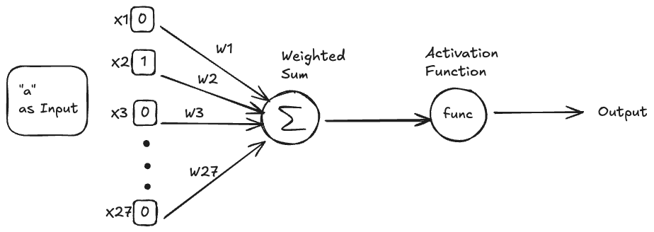
Neuron
A single neuron is made up of the green parts in the diagram above. It generally has 2 components
- A weighted sum with the inputs.
- A non-linear activation function that acts on the weighted sum, say $Func$.
Weights
The weights ($W_1$, $W_2$, …, $W_n$) are the parameters of the function. When we say we will learn the mathematical function, what we mean is that we will learn good values for these parameters that will make the function useful in predicting the $nextCharacter$ when it sees the $previousCharacter$ as input.
Intuitively, we should think of these weights as the strengths that the mathematical function will learn to associate with each connection (link between any particular dimension of the input with the neuron) in the neural network.
I am cheating a bit and jumping ahead here but we’ll soon see that we will finalize the Activation function as well. Then, the only things that will remain a variable are these weights. Hence, our job then would be to tune these weights such that the output of the function becomes useful for us in our given task.
Activation function
The activation function plays the role of adding non-linearity to our function. This is important in order to allow our function to learn arbitrarily complex relationships between the inputs and the outputs it is trying to predict. In our current example, we will see how naturally the need for such a non-linear function arises.
However, for broader generalization, I find it useful to imagine the problem above of finding a boundary between the blue and green dots. In that problem, our input would be a point like $(x, y)$ in the 2-D plane and our output needs to be something that will help us answer if a given point is blue or green. In example $B$ of that problem, ideally the output of our function should be whether given point $(x, y)$ is inside or outside the dotted line circle that encapsulates all blue points since we can use that to infer if the point is blue or green.
Now imagine if our function did not have a non-linear component to it. Our final output function say $Output$ could then only look like a linear combination of $x$ and $y$ at best.
So it would look something like this : \(Output = A*x + B*y + C\)
No matter what values we pick for $A$, $B$ and $C$, there is no way that this output function can tell us if we a given point $(x, y)$ is inside or outside a circle. We need non-linear terms (referencing $x$ and $y$) in order to encapsulate that information.
Putting it all together
So, when we combine all of this, our mathematical function looks like this :
\[Output = Func(W_1*X_1 + W_2*X_2 + …. + W_{27} * X_{27})\]where
- $X_1, X_2,…, X_{27}$ are the different dimensions of the one-hot vector representation of characters.
- $W_1, W_2,…, W_{27}$ are weights corresponding to the connection of each dimension of the input to the neuron.
- $Func$ is our non-linear activation function that operates on the weighted sum of the $Weights$ and $Inputs$.
- $Output$ is the final output of our mathematical function.
This is it. This all a single neuron does. It takes in the multi dimensional input ($X$) and collapses it into a single output number.
Multiple Neurons in Parallel
So far, we know that if we have a single neuron, we can pass it an input (a character, represented like a one-hot vector) and get a single output from it.
But, what if we wanted more than a single output ? What if similar to the input being a vector, we wanted the output to be a vector too ?
But why would we want the output to be a vector ? Well, that is a fair question to ask. And we will get to why soon. For now, if it helps, consider it to just be a thought exercise to understand how can this architecture support a multi dimensional output.
We know that a single neuron gives us a single output. So, if we want a vector as an output, can we just add more neurons ? Well, we can.
Lets see how we can set that up.
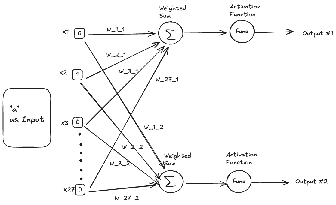
The diagram above shows 2 neurons in parallel, producing 2 outputs.
The way to think about this is that for each input, we first passed it through the first neuron and got one output. Then, we passed the same input through the second neuron and got another output.
Notice that each dimension of the $27$ dimension vector input interacts with each neuron and each such connection has its own Weight. For example, the connection of $X_1$ with $Neuron_1$ has the Weight $W_{11}$ and the connection of $X_2$ with $Neuron_2$ has the Weight $W_{22}$.
This is important because what we’re trying to do is get different outputs from the 2 neurons. If the weights for the connection of $X_i$ with $Neuron_1$ and $Neuron_2$ were the same, then we would get identical outputs from $Neuron_1$ and $Neuron_2$ and that won’t be very useful since there’s no new information there. Our goal is to allow our system to output a multi-dimensional value such that each dimension (the output from each specific neuron) of the output can add new information to help us with solving the problem at hand (predicting the next character).
The example above shows the case for 2 neurons in parallel but we can similarly scale this up to any number of neurons in parallel.
How is all of this useful in predicting the next character?
Well, lets see where we’re at. We started with this :
We have a dataset of names. Somehow we need to use that to come up with a magic function that takes in the previous character and produces an output that we can use to predict the next character.
We can then use this prediction and our algorithm to generate names.
We have made some progress here.
-
From the dataset of names, we have extracted $X$ and $Y$ as our training dataset where $X[i] \to Y[i]$ is a pair of $previousCharacter \to nextCharacter$ association in the given names and each element of $X$ and $Y$ is a one-hot encoded vector of size 27.
- We have set up the structure of our magic math function. It looks like this :
- \[Output = Func(X_1*W_1 + X_2*W_2 + …. + X_{27}*W_{27})\]
- We also know how to extract multiple outputs from our function by using multiple neurons.
- \[Output_1 = Func(X_1*W_{1,1} + X_2*W_{2,1} + …. + X_{27}*W_{27,1})\]
- \[Output_2 = Func(X_1*W_{1,2} + X_2*W_{2,2} + …. + X_{27}*W_{27,2})\]
- …
- \[Output_n = Func(X_1*W_{1,n} + X_2*W_{2,n} + …. + X_{27}*W_{27,n})\]
However, there are still some unknowns here.
- How do we use the $Output$ to predict the next character ?
- We do not know what $Func$ is. We have previously noted that we will finalize this function but we haven’t defined it yet.
- We know that learning this mathematical function means learning good values of $W$. But, How do we find good values of $W$ ?
How do we use the output to predict the next character ?
Before we describe the process of using the $Output$ to predict the next character, lets think a bit more about what our solution should look like.
We know that our algorithm will start with $\langle.\rangle$ and try to predict the first character. Then, it will look at the first character and predict the second character and so on. However, we don’t just want to always predict the same name, right ?
If our process always produces the same $nextCharacter$ when shown a particular $previousCharacter$, then we are guaranteed to always have the same name as the final output.
In order for us to be able to generate different names, we need some randomness in the mix when predicting the $nextCharacter$. But, if we just arbitrarily pick any character at random as the $nextCharacter$ then we’re likely to end up with gibberish that will not look name-like. Ideally, our mathematical function should look at the examples in our training dataset ($X$ and $Y$) and use that to learn the probabilities for each character being picked as the $nextCharacter$.
Then, we could set up a multinomial distribution with those probabilities and pick the next character by sampling from that multinomial distribution.
For example, say the $previousCharacter$ was “$a$” and we knew that the probabilities for the $nextCharacter$ were the following :
- $\langle.\rangle$ : $0\%$
- $a$ : $10\%$
- $b$ : $20\%$
- $c$ : $30\%$
- $d$ : $40\%$
-
$e$ : $0\%$
…
- $z$ : $0\%$
Then, sampling the next character from this probability distribution would be equivalent to if we were randomly choosing a ball from an an urn containing
- $1$ ball labelled $a$
- $2$ balls labelled $b$
- $3$ balls labelled $c$
- $4$ balls labelled $d$
This is great.
We now know that if our mathematical function can take in as input the $previousCharacter$ and output the probabilities for all the 27 possible characters ($\langle.\rangle$, $a$, $b$, $c$, …, $z$) to be chosen as the $nextCharacter$, then we know how to use those probabilities to randomly generate the $nextCharacter$.
This tells us that we need the $Output$ to satisfy the following conditions:
-
We need to generate $27$ numbers, i.e., the probabilities for the $27$ possible characters that can be chosen as the $nextCharacter$.
-
We need the $27$ output numbers to form a probability distribution. This means
- Each of those $27$ numbers should lie between $0$ and $1$.
- If we sum up all $27$ numbers, they should sum up to $1$.
Ah, but we know how to generate $27$ outputs. We can do that by having $27$ neurons in parallel, with each neuron generating one number as the output. Lets refresh what that means for our mathematical function.
We know our inputs look like one-hot vectors. So, say, $x$ is an input which represents the character “$a$”.
So, $x = [0, 1, 0, 0, …, 0]$ with the size of $x$ being 27. This means that $x_0 = 0$, $x_1 = 1$, $x_2 = 0$, …, $x_{26} = 0$
We also know that each dimension of $x$, i.e., each $x_i$ will interact with each $Neuron_j$ via its own weight. Thus, we’ll have $27$ dimensions of the input interacting with $27$ Neurons, each connection having its own weight. We can represent these weights as a $27$ X $27$ matrix $W$ such that $W[i][j]$ represents the weight of the connection between $x_i$ and $Neuron_j$.
Finally, we know that we’ll have $27$ numbers in the output, one output from each Neuron. Lets represent that via the vector $Output$ such that $Output[j]$ is the output from $Neuron_j$.
So, our mathematical function looks like this now :
$Output[j] = Func(X_0 * W[0][j] + X_1 * W[1][j] +$ $… + X_{26} * W[26][j])$
where $j$ $\in$ ${0, 1, …, 26}$
In addition, we need $Output[j]$ for $j$ $\in$ ${0, 1, …, 26}$ to form a probability distribution since we want $Output[j]$ to be the probability of picking the character indexed by $j$ ($\langle.\rangle = 0$, $a = 1$, $b = 2$, …, $z = 26$) as the next character.
This means
- $0 <=$ $Output[j] <=$ $1$ for $j$ $\in$ ${0, 1, …, 26}$.
- $\sum_{j=0}^{j=26}$ $Output[j] = 1$.
We still haven’t defined what $Func$ is yet. Lets see how we can choose an appropriate definition for $Func$ such that we can ensure that $Output[j]$ for $j$ $\in$ ${0, 1, …, 26}$ forms the probability distribution that we need.
Choosing an appropriate non-linear activation function
We know that we have a mathematical function takes as input the $previousCharacter$ ($X = [X_0, X_1, X_2, … , X_{26}]$) and generates an output that looks like this :
$Output[j] = Func(X_0 * W[0][j] + X_1 * W[1][j] +$ $… + X_{26} * W[26][j])$
where $j$ $\in$ ${0, 1, …, 26}$
and we know that we want $Output[j]$ to be the probability of picking the character indexed by $j$ ($\langle.\rangle = 0$, $a = 1$, $b = 2$, …, $z = 26$) as the next character.
Our job now is to pick an appropriate definition for $Func$ such that
- we can enforce that $Output[j]$ forms a probability distribution
- we can interpret $Output[j]$ to be the probability of picking the character indexed by $j$ ($\langle.\rangle = 0$, $a = 1$, $b = 2$, …, $z = 26$) as the next character.
In order to develop an intuition for how we can interpret $Output[j]$ to be the probability of picking the character indexed by $j$ ($\langle.\rangle = 0$, $a = 1$, $b = 2$, …, $z = 26$) as the next character, lets first look at an alternate way of solving our problem that does not use Neural Networks.
Alternate Solution to the Name generation problem
We’re still trying to solve the same problem here.
- We have a dataset of names.
- We are trying to generate new names.
- Our strategy is still to look at the $previousCharacter$ and then predict the $nextCharacter$.
- From the dataset of names, we will extract ($X$, $Y$) as our training examples where $X[i] \to Y[i]$ is a pair of $previousCharacter \to nextCharacter$ association in the given names.
However, we’re taking a detour from the world of Neural Networks for a bit.
Instead, lets create a counting based Matrix $C$ of size $27$ x $27$.
| $\langle.\rangle$ | $a$ | $b$ | $c$ | … | … | $z$ | |
|---|---|---|---|---|---|---|---|
| $\langle.\rangle$ | $C_{0,0}$ | $C_{0,1}$ | $C_{0,2}$ | $C_{0,3}$ | $C_{0,26}$ | ||
| $a$ | $C_{1,0}$ | $C_{1,1}$ | $C_{1,2}$ | $C_{1,3}$ | $C_{1,26}$ | ||
| $b$ | $C_{2,0}$ | $C_{2,1}$ | $C_{2,2}$ | $C_{2,3}$ | $C_{2,26}$ | ||
| $c$ | $C_{3,0}$ | $C_{3,1}$ | $C_{3,2}$ | $C_{3,3}$ | $C_{3,26}$ | ||
| … | |||||||
| … | |||||||
| $z$ | $C_{26,0}$ | $C_{26,1}$ | $C_{26,2}$ | $C_{26,3}$ | $C_{26,26}$ |
Lets assume that we’ve indexed the characters as :
- $\langle.\rangle = 0$
- $a = 1$
- $b = 2$
- …
- $z = 26$
Each cell of this matrix, $C[i][j]$ is the count of how often we’ve seen the character indexed by $i$ followed by the character indexed by $j$ in our training examples ($x$, $y$) where $x \to y$ is a pair of $previousCharacter \to nextCharacter$ association in the given names.
For example, if one of the names in the dataset was alex, then we have the following ($x$, $y$) pairs from alex :
- $\langle.\rangle \to a$
- $a \to l$
- $l \to e$
- $e \to x$
- $x \to \langle.\rangle$
If we change these pairs to instead reference the indexes for the characters, they would be
- $0 \to 1$
- $1 \to 12$
- $12 \to 5$
- $5 \to 24$
- $24 \to 0$
And so, each of these pairs would increase the counts in the corresponding cells in the matrix $C$ by $1$.
- $C[0][1]$ $\mathrel{+}= 1$
- $C[1][12]$ $\mathrel{+}= 1$
- $C[12][5]$ $\mathrel{+}= 1$
- $C[5][24]$ $\mathrel{+}= 1$
- $C[24][0]$ $\mathrel{+}= 1$
Similarly, we can iterate over all the names in the dataset and populate the matrix $C$.
Now, lets think about what each row of $C$ tells us. Lets take the row corresponding to “$a$”, i.e row $C[1]$.
Each element of that row, $C[1][j]$ for $j$ $\in$ ${0, 1, …, 26}$, is the count of how often we’ve encountered the pair ($a \to$ Character indexed by $j$) in our dataset of names.
Now, lets say that if we knew that the $previousCharacter$ was “$a$” and we wanted to predict the $nextCharacter$.
We have previously noted that if we could somehow figure out the probabilities for all the 27 possible characters ($\langle.\rangle$, $a$, $b$, $c$, …, $z$) to be chosen as the $nextCharacter$, then we know how to use those probabilities to randomly generate the $nextCharacter$.
Is there a way that we can use the row $C[1]$ to generate those probabilities ?
Note that the row $C[1]$ has 27 columns, with each column in that row denoting the count of how often the character indexed by that column has followed the character “$a$” in our dataset of names.
Lets call $Sum[1]$ to be the sum of all entries in row $1$, i.e., the sum of the counts of all the characters that have followed “$a$” in our dataset of names.
Hence, $Sum[1]$ = $\sum_{j=0}^{j=26}$ $C[1][j]$
Then, the probability of the character indexed by $j$ to be chosen as the $nextCharacter$ to follow $a$, would simply be
$Prob[1][j]$ = $\frac{C[1][j]}{Sum[1]}$ for $j$ $\in$ ${0, 1, …, 26}$
Basically, all we have done is :
- Looked at how often a particular character follows $a$ in our dataset of names
- Assign the probability of choosing that character as the character to follow $a$ in our generated name by comparing its count relative to the counts of all the characters that have followed $a$ in our dataset of names.
Once we have these probabilities, we know how to how generate the next character.
Back to defining the non-linear activation function
The critical thing to understand from the counting based solution we explored above is how we interpreted the rows of the matrix $C$.
The row corresponding to “$a$”, i.e row $C[1]$ had 27 entries, each of them maintaining the count of often the character indexed by that column followed “$a$” in the dataset of names. We then used these counts to convert them into probabilities for each character by normalizing the individual counts against the sum of the counts of every character that followed “$a$” in our dataset of names.
We were able to do this because we were able to interpret the 27 entries in the row $C[1]$ as the strengths of each particular character being chosen as the next character to follow “$a$” since they reflected how often we have already seen those characters follow “$a$” in our dataset of names.
So, with that in mind, lets see if we can create a similar analogy in our Neural Network setup that can help guide us to define our Activation Function.
It turns out that we have a matrix in our neural network setup that is fairly similar to the matrix $C$ that we had in our counting based solution.
Lets again index our characters as following :
- $\langle.\rangle = 0$
- $a = 1$
- $b = 2$
- …
- $z = 26$
We have a mathematical function that takes as input the $previousCharacter$ ($X = [X_0, X_1, X_2, … , X_{26}]$) and generates an output that looks like this :
$Output[j] = Func(X_0 * W[0][j] + X_1 * W[1][j] +$ $… + X_{26} * W[26][j])$
where $j$ $\in$ ${0, 1, …, 26}$
Remember, we want $Output[j]$ for $j$ $\in$ ${0, 1, …, 26}$ to form a probability distribution since we want $Output[j]$ to be the probability of picking the character indexed by $j$ as the next character when the $previousCharacter$ is $X$.
There are exactly 27 different possible values for the Input $X$.
- $\langle.\rangle = [1,0,0,…,0]$
- $a = [0,1,0,…,0]$
- $b = [0,0,1,…,0]$
- …
- $z = [0,0,0,…,1]$
Lets index these as following :
- $[1,0,0,…,0] = 0$
- $[0,1,0,…,0] = 1$
- $[0,0,1,…,0] = 2$
- …
- $[0,0,0,…,1] = 26$
Now, lets define a matrix $P$ as following:
$P[i][j] = Output[j] = Func(X_0 * W[0][j] + X_1 * W[1][j] +$ $… + X_{26} * W[26][j])$
where $j$ $\in$ ${0, 1, …, 26}$
and $X$ = i (as referenced by the indexing defined above)
In other words, $P[i][j]$ is the value of the $Output$ from $Neuron_j$ for the Input, i.e., the $previousCharacter$, being set to the character indexed by $i$.
So our matrix $P$ is of size $27$ x $27$.
| $\langle.\rangle$ | $a$ | $b$ | $c$ | … | … | $z$ | |
|---|---|---|---|---|---|---|---|
| $\langle.\rangle$ | $P_{0,0}$ | $P_{0,1}$ | $P_{0,2}$ | $P_{0,3}$ | $P_{0,26}$ | ||
| $a$ | $P_{1,0}$ | $P_{1,1}$ | $P_{1,2}$ | $P_{1,3}$ | $P_{1,26}$ | ||
| $b$ | $P_{2,0}$ | $P_{2,1}$ | $P_{2,2}$ | $P_{2,3}$ | $P_{2,26}$ | ||
| $c$ | $P_{3,0}$ | $P_{3,1}$ | $P_{3,2}$ | $P_{3,3}$ | $P_{3,26}$ | ||
| … | |||||||
| … | |||||||
| $z$ | $P_{26,0}$ | $P_{26,1}$ | $P_{26,2}$ | $P_{26,3}$ | $P_{26,26}$ |
Lets look at what each row of the Matrix $P$ tells us. Lets take the row corresponding to the input (the $previousCharacter$) being “$a$”, i.e row $P[1]$.
Each element of that row, $P[1][j]$ for $j$ $\in$ ${0, 1, …, 26}$ is the $Output$ produced by $Neuron_j$ when it is fed the character $a$ as input. We know that we want this value to be the probability of choosing the character indexed by $j$ as the next character when our Neural Network is fed the character $a$ as input.
Thus, the row corresponding to the input (the $previousCharacter$) being “$a$” in the matrix $P$ is simply the probabilities of each character being chosen as the next character after “$a$”.
$P[1][j] = Output[j] = Func(X_0 * W[0][j] + X_1 * W[1][j] +$ $… + X_{26} * W[26][j])$
Where $[X_0, X_1, X_2, …, X{26}] = [0,1,0,…,0]$
Lets look at the input to $Func$, i.e., $X_0 * W[0][j] + X_1 * W[1][j] +$ $… + X_{26} * W[26][j]$
This value is the raw output from the Neuron, i.e., the output from the neuron before applying the Activation function on it. In neural network terminology, this value is known as $Logits$ of the Neuron.
$Logits[1][j] = X_0 * W[0][j] + X_1 * W[1][j] +$ $… + X_{26} * W[26][j]$
where $j$ $\in$ ${0, 1, …, 26}$
and $[X_0, X_1, X_2, …, X_{26}] = [0,1,0,…,0]$
Remember that we still haven’t decided how we’re going to pick the values of the matrix $W$. But, for now, assume that we have some mechanism to pick the values of $W$ such that the $Logits[1][j]$ can be interpreted as the strength that our model has learned of choosing the character indexed by $j$ to be the $nextCharacter$ when the model is shown “$a$” as the input.
In the counting based solution, the values $C[1][j]$ were fairly similar to the values $Logits[1][j]$ that we have arrived at here. Both were 27 values that were each interpreted as the strength that the solution has learned of choosing the character indexed by $j$ to be the $nextCharacter$ when the model is shown “$a$” as the input.
In the counting based solution, we were able to convert $C[1][j]$ into probabilities for each character by normalizing the individual counts against the sum of the counts of every character that followed “$a$” in our dataset of names.
$Prob[1][j]$ = $\frac{C[1][j]}{Sum[1]}$ for $j$ $\in$ ${0, 1, …, 26}$
What stops us from doing the same with $Logits[1][j]$ ?
Well, We knew that $C[1][j]$ for $j$ $\in$ ${0, 1, …, 26}$ were all non-negative numbers since they were counts. However, $Logits[1][j]$ could very well be negative numbers.
So, we need a way to convert $Logits[1][j]$ to be non-negative numbers.
Consider $E_{logits}[1][j]$ = ${e}^{logits[1][j]}$
We know that ${e}^x \geq 0$ for every value of $x$.
In addition, ${\rm e}^x$ is a monotonic function.
Thus, if $logits[1][j_1] \geq logits[1][j_2]$, then, $E_{logits}[1][j_1] \geq E_{logits}[1][j_2]$
This implies that if $Logits[1][j]$ could be interpreted as the strength that the solution has learned of choosing the character indexed by $j$ to be the $nextCharacter$ when the model is shown “$a$” as the input, then we could also interpret $E_{logits}[1][j]$ as the same thing.
Hence, $E_{logits}[1][j]$ = ${\rm e}^{logits[1][j]}$ is a set of 27 non-negative numbers that can be interpreted as the strength that the solution has learned of choosing the character indexed by $j$ to be the $nextCharacter$ when the model is shown “$a$” as the input.
Now, we can do the same thing with $E_{logits}[1][j]$ that we did with $C[1][j]$ to convert them into probabilities.
Define $Sum_{logits}[1] =$ $\sum_{j=0}^{j=26}$ $E_{logits}[1][j]$
Then, $P[1][j] = \frac{E_{logits}[1][j]}{Sum_{logits}[1]}$ = $\frac{e^{logits[1][j]}}{\sum_{j=0}^{j=26}{e^{logits[1][j]}}}$
So, $P[1][j]$ is the probability of choosing the character indexed by $j$ as the next character when our Neural Network is fed the character $a$ as input.
But, from our definition, we know that
$P[1][j] = Func(X_0 * W[0][j] + X_1 * W[1][j] +$ $… + X_{26} * W[26][j])$ $= Func(logits[1][j])$
So, $Func(logits[1][j])$ = $\frac{e^{logits[1][j]}}{\sum_{j=0}^{j=26}{e^{logits[1][j]}}}$
Hence, we now know what our $Func$ should be defined as.
$Func(x) =$ $\frac{e^{x}}{\sum_{j=0}^{j=26}e^{x}}$
This particular activation function is known as the “Softmax” function. It is known as softmax because instead of outputting just the maximum element from a set of elements, it instead outputs a softer version of that by outputting the probability distribution for the set instead.

How do we find good values of W ?
First, lets recap all that we have built up so far.
- From the dataset of names, we have extracted $X$ and $Y$ as our training dataset where $X[i] \to Y[i]$ is a pair of $previousCharacter \to nextCharacter$ association in the given names and each element of $X$ and $Y$ is a one-hot encoded vector of size 27.
- We have a neural network setup consisting of 27 neurons, each connected to the 27 dimensions of the input and each connection having a particular weight, leading to the Weight matrix $W$ of size $27$ x $27$. We need to learn the value of this $W$ matrix.
- The input to this neural network is the $precedingCharacter$.
- For any given Input, each of the 27 neurons produces an output.
- We have indexed the characters as ($\langle.\rangle = 0$, $a = 1$, $b = 2$, …, $z = 26$).
- We have defined
- $Logits[i][j] = X_0 * W[0][j] + X_1 * W[1][j] +$ $… + X_{26} * W[26][j]$
- Where $j$ $\in$ ${0, 1, …, 26}$ iterates over each neuron.
- and $[X_0, X_1, X_2, …, X_{26}]$ is the one-hot vector representation of the input character indexed by $i$.
- We have defined $P[i][j]$ as the output of $j’th$ Neuron of the neural network when the input $[X_0, X_1, X_2, …, X_{26}]$ is the one-hot vector representation of the input character indexed by $i$.
- $P[i][j]$ = $\frac{e^{logits[i][j]}}{\sum_{j=0}^{j=26}{e^{logits[i][j]}}}$
- We know that $P[i][j]$ for $j$ $\in$ ${0, 1, …, 26}$ , i.e., the output from all the neurons for a given input forms a probability distribution.
- We have decided to interpret $P[i][j]$ as the probability of choosing the character indexed by $j$ as the next character when our Neural Network is fed the character indexed by $i$ as input.
- Once we know the values for $P[i][j]$ for all $i$ and $j$
There’s only 2 things here that we still need to work on.
We still don’t know how to learn the values of the Matrix $W$.
While we have decided to interpret $P[i][j]$ as the probability of choosing the character indexed by $j$ as the next character when our Neural Network is fed the character indexed by $i$ as input, there is no reason yet to believe that this interpretation is actually valid.
How do we know that the values of $P[i][j]$ are actually informed by the $X[i] \to Y[i]$ pairs of $previousCharacter \to nextCharacter$ associations in the names in our dataset ?
Well, both these problems are fairly linked. When we said that we’ll interpret $P[i][j]$ as the probability of choosing the character indexed by $j$ as the next character when our Neural Network is fed the character indexed by $i$ as input, we made an assumption that we can choose the values of $W$ to be such that the interpretation makes sense.
So, lets see how we can do that.
We need a way to evaluate if we have good values of W
Say we picked a random value for the $W$ matrix. We can then calculate $P[i][j]$ for all $i$ and $j$. We already have our algorithm that we could then use to generate the names we want.
But, how do we evaluate the quality of our predicting model ? A good model would be one that predicted names that resembled the ones in our dataset.
We need a mathematical way to represent this quality. Ideally, we need to come up with a number that could be used to represent this quality so that we could then shift our focus to playing around with the values of $W$ and try to optimize for the the quality of the model.
In Neural network terminology, we call this number the Loss function of the neural network. The semantics for the Loss function is that it should be a function of the parameters of the network ($W$ in our case) and it should be $\geq 0$. The lower the value of the Loss function, the better quality model we have.
Negative Log Likelihood as the Loss function
Remember that we want to interpret $P[i][j]$ as the probability of choosing the character indexed by $j$ as the next character when our Neural Network is fed the character indexed by $i$ as input. And we know that the values of $P[i][j]$ is a function of $W$.
What is a way that we could validate that our chosen value for the matrix $W$, which would determine the values of $P[i][j]$, supports our interpretation ?
Well, we already have a dataset of names. Lets say it has the word alex in there. If we have learnt our mathematical function well, then the probability for our model to predict the word alex should be high since we do want our model to predict names that are similar to the names in our dataset.
As per our algorithm, our model will predict the name alex if
- It predicts $a$ when it sees $\langle.\rangle$ as the input.
- It predicts $l$ when it sees $a$ as the input.
- It predicts $e$ when it sees $l$ as the input.
- It predicts $x$ when it sees $e$ as the input.
- It predicts $\langle.\rangle$ when it sees $x$ as the input.
Hence, $Prob(alex)$ = $P[0][1] * P[1][12] * P[12][5] * P[5][24] * P[24][0]$
So, if we want $Prob(alex)$ to be high, we would want $P[0][1] * P[1][12] * P[12][5] * P[5][24] * P[24][0]$ to be high.
We can do a similar exercise for every name in the dataset. From the dataset of names, we had extracted $X$ and $Y$ as our training dataset where $X[i] \to Y[i]$ is a pair of $previousCharacter \to nextCharacter$ association in the given names.
We also know that
$Prob(word)$ = $\prod P[index(X[i])][index(Y[i])]$ for all $(X[i], Y[i])$ pairs in the word.
where $index(X[i])$ is the index of the character $X[i]$ as per our definition of the index.
Claim : We should choose the value of $W$ such that it tries to maximize the product of $P[index(X[i])][index(Y[i])]$ for all $(X[i], Y[i])$ pairs in our dataset.
Lets think about what this means.
The product of $P[index(X[i])][index(Y[i])]$ for all $(X[i], Y[i])$ pairs in our dataset is equal to the product of the Probabilities of all the names in our dataset being predicted by our model. Given that our model is being trained on these names, it should be expected that the model’s probability to generate the names within the dataset should be high.
In addition, this framing of the problem of choosing $W$ makes our interpretation of $P[i][j]$ valid. If the product of $P[index(X[i])][index(Y[i])]$ for all $(X[i], Y[i])$ pairs in our dataset is high, that means that the $P[index(X[i])][index(Y[i])]$ for any given pair of $(X[i], Y[i])$ that is found in our dataset is high.
This is exactly what we would want to support our interpretation of $P[i][j]$. Since all we have in terms of examples are the names in our dataset, in order to be confident that $P[i][j]$ can indeed be interpreted as the probability of choosing the character indexed by $j$ as the next character when our Neural Network is fed the character indexed by $i$ as input, the values of $P[i][j]$ should be high for the examples already found in the dataset as they come from words that we know are names.
So, now we know what it means for us to “pick good values of $W$”.
A good value of $W$ will try to maximize the product of $P[index(X[i])][index(Y[i])]$ for all $(X[i], Y[i])$ pairs in our dataset.
Lets Define :
$Likelihood(dataset)$ = $\prod$ $P[index(X[i])][index(Y[i])]$ for all $(X[i], Y[i])$ pairs in our dataset
Note that Likelihood is a well defined term in statistical modeling. We have not gone into detail in explaining what it means since for our purposes we can just assume the definition above (without other context) and work with it.
Thus, what we’re trying to do is choose a value of $W$ that maximizes $Likelihood(dataset)$.
So, lets define the Loss Function for our network.
Recall that the Loss Function has the semantics that it is $\geq 0$ and we have the goal of minimizing the Loss Function.
Now, Maximizing the $Likelihood(dataset)$ is equivalent to Minimizing $-1 * Likelihood(dataset)$
$Likelihood(dataset)$ is made up by multiplying lots of Individual probabilities. Since each probability is a number between $0$ and $1$, multiplying lots of such terms can lead to very small and unwieldy numbers.
In order to avoid that problem, we can instead work with $\log_{e}(Likelihood(dataset))$.
Remember that $- \infty <$ $\log_{e}(x) \leq 0$ for $0$ $<$ $x$ $\leq$ $1$.
Also, $\log_{e}(x)$ is a monotonic function. Thus, minimizing $f(x)$ is the same as minimizing $\log_{e}(f(x))$.
Thus, we have now converted our problem of
- maximizing $Likelihood(dataset)$
into the problem of
- minimizing $-1 * \log_{e}(Likelihood(data))$
Remember the following:
-
$Likelihood(dataset)$ = $\prod$ $P[index(X[i])][index(Y[i])]$ for all $(X[i], Y[i])$ pairs in our dataset
-
$\log_{e}(a * b * c) = \log_{e}(a) + \log_{e}(b) + \log_{e}(c)$
So, $\log_{e}(Likelihood(dataset))$ = $\log_{e}(\prod$ $P[index(X[i])][index(Y[i])]$) = $\sum \log_{e}(P[index(X[i])][index(Y[i]))]$
where the summation is over all $(X[i], Y[i])$ pairs in the dataset
Thus, our problem of
- minimizing $-1 * \log_{e}(Likelihood(data))$
is equivalent to
- minimizing $-1 * \sum \log_{e}(P[index(X[i])][index(Y[i]))]$
Also notice that
- $-1 * \sum \log_{e}(P[index(X[i])][index(Y[i]))]$ $\geq 0$
Let the total number $(X[i], Y[i])$ pairs in the dataset be $N$.
In order to be able to operate on fairly large datasets without the risk of
- $-1 * \sum \log_{e}(P[index(X[i])][index(Y[i]))]$
turning into a very large number and to be able to compare the values of the loss function independent of the size of the dataset, we can instead work on
- the average value of $-1 * \sum \log_{e}(P[index(X[i])][index(Y[i]))]$ over the entire dataset.
Thus, we can convert our problem
- minimizing $-1 * \sum \log_{e}(P[index(X[i])][index(Y[i]))]$
into
- minimizing $\frac{-1}{N} * \sum \log_{e}(P[index(X[i])][index(Y[i]))]$
Thus, our loss function for the network is :
$\frac{-1}{N} * \sum \log_{e}(P[index(X[i])][index(Y[i]))]$
where the summation is over all $(X[i], Y[i])$ pairs in the dataset
and $N$ = Total number of $(X[i], Y[i])$ pairs in the dataset.
Gradient Descent as the Optimization mechanism
We have most of the infrastructure in place now.
- Say we arbitrarily pick some value of the matrix “$W$”.
- We know how to use $W$ to calculate the value for the loss function of the model.
- We also know that if the loss function is a high number, that indicates that our model’s quality is not great and we need to change “$W$” in order to reduce the loss function.
However, we cannot just randomly play around with the value of “$W$” and hope that we land at a small value for the loss function. I mean you could, but good luck to you in that case.
Instead, we can use a technique called “Gradient Descent” to optimize the value of our loss function by iteratively changing the value of “$W$”.
Remember that our loss function is :
$\frac{-1}{N} * \sum \log_{e}(P[index(X[i])][index(Y[i]))]$
where the summation is over all $(X[i], Y[i])$ pairs in the dataset
and $N$ = Total number of $(X[i], Y[i])$ pairs in the dataset.
For a given dataset, the pairs of $(X[i], Y[i])$ are fixed.
Hence, our loss function is a function of $W$. Also note that the loss function is a differentiable function of $W$ since every mathematical operation done to define it is a differentiable operation.
We are now going to introduce the crux of why Gradient Descent as a technique works, but we’re not going to prove it here. Feel free to read more about it on your own.
FACT : if $f(x)$ is differentiable at $x$, then $f(x + \alpha * f’(x)) > f(x)$ where $\alpha$ is a small positive number and $f’(x)$ is the derivative/gradient of $f$ at $x$.
In other words, if $f(x)$ is differentiable at $x$, then if we take a small step in the direction of the gradient at $x$, then the function’s value increases. This implies that if we take a small step in the opposite direction of the gradient at $x$, then the function’s value decreases.
We can use this fact to optimize our loss function.
Consider the following algorithm:
- Step 1 : Pick an arbitrary value of $W$.
- Step 2 : Pick a value of $M$ , say $M = 10,000$
Run the following steps in a loop for $M$ times:
- Step 3 : Calculate the loss function of the network. This is known as the forward pass of the neural network.
- Step 4 : Calculate the gradient of the loss function with respect to $W$. Lets call it $grad$.
- Step 5 : Determine a small step function, i.e., the value of “$\alpha$” which will be the size of the step we take.
- Step 6 : Update $W$ = $W$ - $\alpha$ $*$ $grad$. Steps 4, 5 and 6 are known as the backward pass of the neural network.
Step 6 ensures that with each iteration, the value of our loss function should decrease, which is exactly what we want.
Practically, we would want to run the steps 3 to 6 until we see the value of the loss function converge near a particular value.

